In this section, you will learn how to use a few tools from the phylogeny-analysis program Phylip to make a phylogenetic tree by a more rigorous method, called neighbor joining.
Point your browser to http://bioweb2.pasteur.fr/intro-en.html and click Phylogeny.
This is one home of the program Phylip, One of the most rigorous tools for constructing phylogentic trees from aligned sequences.
Under Computation of Distance, Phylip, click protdist.
You are about to run protdist, a program that computes the "distance", or the quantitative amount of difference, of protein sequences from each other. These so-called distance matrices will be used by Phylip to construct your tree. The input to protdist is the multiple-sequence alignment you made using Clustalw (file: OpsinMSAEdited.txt)
Enter your email into the top box.
In the alignment file box, paste your edited mutiple sequence alignment from ClustalW (OpsinMSAEdited.txt).
Under Bootstrap Options, make these settings:
Leave other settings as you found them, and click Run.
protdist constructs distance matrices by a process called "bootstrapping". Bootstrapping is a bias-reducing procedure in which protdist builds an alignment of pseudosequences by picking residue positions at random and stringing the residues at those positions together until the sequence is the same length as the original ClustalW alignment. From this pseudosequence alignment, protdist determines the relative number of sequence difference among the five proteins, as determined from a random sampling of their sequences. The result of the process is a called distance matrix, and you will see it soon. This process is repeated, 100 times in our case, to make 100 distance matrices. The tree we will ultimately produce represents a consensus of the 100 matrices.
On the results page, look in the outfile window to see the 100 matrices containing numbers that represent the relative number of differences among the five sequences. Each matrix has the sequence names in the first column, and you should imagine that these sequence names are also the headings for the remaining columns. The number at the intersection of the row Blue and the column with the imaginary heading Peropsin gives the relative magnitude of the sequence differences between the blue opsin and peropsin. The matrices have zeros on the diagonal because each pseudosequence is identical to itself. Click the Save button to save the entire file of 100 matrices. The file is automatically downloaded with the name protdist.outfile.txt. Transfer the file to a convenient place.
Clicking the Back button of your browser from a results page takes you back to the Phylogeny page. Under Distance Matrix Method programs, Phylip click neighbor. Read the lists carefully: don't pick "weighbor".
Into the Distance matrix File window, paste the contents of the file protdist.outfile.txt. Under Bootstrap options make these settings:
Scroll down to Other options.
This entry area gives you the option of designating an outgroup for the root of your tree. An outgroup is the sequence you think is most distant from the others, possibly the common ancestor of all. We don't know that in this case, so leave the default of 1.
At the top of the page, click Run.
On the results page, the Newick file you need to make the tree is neighbor.outtree. Copy and save it as PhylipTreeData.txt.
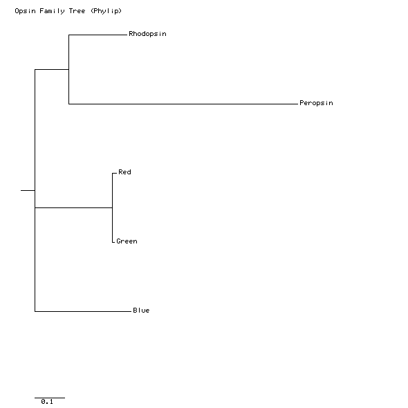
By scrolling down in the consense.outfile window, you can see the consensus tree, printed in a simple text format. This tree is listed as "unrooted", meaning that we do not know the ancestor of all these sequences. We learn from this tree which sequences are most alike and which are most different. We also learn how often the connections of this tree were made the same way in the 100 trees made from those 100 difference matrices. The numbers on the branches indicate the number of times that partition of the species into the two sets separated by that branch occurred among the 100 trees. For example, the separation of Red and Green from the other three, indicating that Red and Green are more similar to each other than to the other three, occurred in all 100 trees. The separation of Blue and Peropsin from the other three occurred in only 53 of the 100 trees. In the other 47 trees, Rhodopsin and Peropsin were separated from the other three. (Can you extract this information from this file?) In the tree branching shown, the majority rules, and the results of 47 of the trees are discarded.
Note: Your results may be slightly different from mine. Because of the random choices made in constructing the tree, the percentages in the paragraph above my vary. I have gotten as high as 82% consensus on the separation of Blue and Peropsin from the other three.
Using what you learned in the previous section, go to http://iubio.bio.indiana.edu/treeapp/treeprint-form.html and produce a tree from data in your file PhylipTreeData.txt.
Here is my tree:
Interpreting a tree is not as simple as interpreting the types of trees that you see in textbooks. The Phylip tree apears to say that the divergence of Blue from Rhodopsin came before the divergence of Rhodopsin from Peropsin. But remember that this tree is unrooted; we did not specify which protein we think is the progenitor of the others. The tree-printing program automatically puts a little root on the tree, but that line is not necessarily the beginning or "bottom" of the tree. We can start from any branch and read the tree as if that were the first branching event on the tree. What the tree does tell us is which sequences are the most similar. Clearly, Red and Green are the most similar pair, and Blue is more similar to rhodopsin than is is to peropsin.
Next, you will use some of the latest tools to make a multiple-sequence alignment (Tcoffee) and a tree (PhyML). These programs are even more powerful, but with power comes somewhat less transparency, and a cost in speed. The experts say that the results are better, but we pretty much just have to take their word for it. PhyML also uses a bootstrapping approach, but with greater redundancy than Phylip. The really neat thing about PhyML is that it lets you play with the tree in many ways, including changing roots interactively.
For making a multiple-sequence alignment with Tcoffee, you need raw FASTA files. To get them,
Point your browser to http://tcoffee.vital-it.ch/cgi-bin/Tcoffee/tcoffee_cgi/index.cgi?stage1=1&daction=TCOFFEE::Regular
Paste your FASTA data into the space provided. Enter your email address. Click Submit. That's all there is to it. After what is usually a short delay, a results page appears. It provides links to your multiple-sequence alignment in several formats. (You might find it interesting to compare the alignment from Tcoffee to the one you got from ClustalW. This is easiest to do with the Tcoffee file clustalw_aln.) The file you want for producing a tree is labeled phylip, which provides the alignment in Phylip format, which is needed for PhyML. Click phylip to see this file, select all the text displayed, and copy it. Paste it into a text file, 5Opsins4PhyML.txt).
Point your browser to http://atgc.lirmm.fr/phyml/
PhyML uses maximum-likelihood methods, which are based on very powerful (but obscure) Bayesian statistics, to calculate the tree that has the highest probability of showing the correct relationship among the aligned sequences. Maximum-likelihood methods are among the most highly respected means of making decisions when you must navigate a minefield of probability-based choices to arrive at a either a single best decision, or a small group of similar good ones (X-ray crystallographers use it to decide which data to use, and which to exclude, when trying to build a model of a protein from diffraction data). As the availability of such methods has grown, so has the number of people for whom they are completely black boxes. When you use a black-box method, you must be careful to compare the results with everything else you know about the subject. A surprising result might be a genuine discovery, or it might be just wrong. It is a result to test further, not to accept blindly.
Now put this black box to work.
In the PhyML form, make these settings:
Sequences: File; then click Choose File, and choose the phylip file you saved from the Tcoffee output.
Data Type: Amino Acids
Sequence File: Interleaved
Number of data sets: 1, also click Perform bootstrap
Number of bootstrap data sets: 100 (do not click Print bootstrap info.)
Enter your name, country, email, and type of computer you are using. Then click Execute and email results. It might take as much as an hour for the results to arrive.
Your email will contain a link to your tree. Click the link, read about the tree viewer, and click View tree.
If you computer is properly configured to run Java applets, the ATV Viewer will appear with your tree, along with many tools for controlling its display. Each tree tip contains the UniProt accession number of an opsin sequence. You can display additional information on the tree by clicking one of the squares on the right-hand menu. Click branch length values to add the relative distances along the branches. Next click Editable to allowing you to play with the display. Under click on node to: click display/edit information. Then click the node (blue square) at sp|O14718| and change the sequence name to peropsin, and click Write to tree. Change the other sequence names (see previous section) to red opsin, green opsin, blue opsin, and rhodopsin.
Next, under click on node to: click root/reroot. You will now set an outgroup for the tree. Because peropsin is the only member of this group that is not known to be directly involved in vision, make the (arbitrary) assumption that it was the first to split off from the group by rooting the tree with peropsin. Make it the outgroup of the tree by clicking on the node (blue square) next to peropsin. You can also pick swap children and click branch nodes to switch display positions for a branch, a purely cosmetic operation, but one that sometimes makes it much easier to interpret the tree. Adjust the window size or the zoom settings so that all information is clearly displayed. Then use a screen save command to save an image of the tree.
To capture pictures on my Macintosh computer, I use the very handy (and very old) shift-command-4, which allows me to select a rectangle on the screen and then saves a .png file of my selection to the desktop with the name Picture 1.
Here's the tree I made according to these instructions:
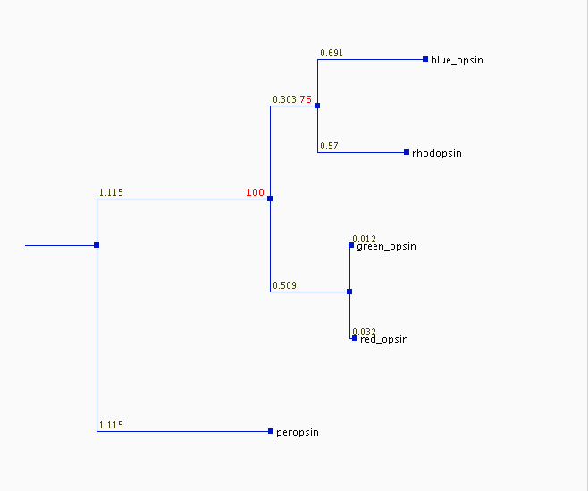
If it is true (and we don't know) that the proper base for this tree is divergence of the peropsin gene from those of the other opsins, then the tree tells the following superficially plausible story of an ancestral gene produced the opsin genes we find today. Peropsin first diverged from a progenitor that was destined to become the parent of all the visual opsins (the progenitor might already have been a primitive visual pigment). Later, a color-specific opsin diverged from the primitive rhodopsin (branch labeled 100). Next, the rhodopsin line split (75), ultimately producing the blue opsin and today's rhodopsin. Most recently, the first color-sensitive opsin gave rise to the red and green opsins, which are still by far the most similar pair of opsins. Each branch probably represents a gene duplication, and one copy gene retained the original function, while the other gradually mutated to produce a protein of new function. Gene duplications are common, but evolution of one copy into something useful is probably far less common; most duplicates end up as nonfunctional pseudogenes.
Again, remember that you are merely scratching the surface of the tools introduced in this tutorial. To make and defend decisions about phylogenetic relationships. you need to know more about these tools and the underlying computations. See the last section of the tutorial for more on this subject.