Please wait for the entire file to load before clicking links. It's a biggie.
Gale Rhodes
Contact Information
Crystallographic, NMR, homology, and other models of biomolecules are greeted by a research audience anxious to use these models to interpret results of their research on molecular function. With the ready availability of a thousands of models comes the need to understand how these models are obtained, and to be aware of the strengths and weaknesses of each method of "structure determination."
No one has ever seen a molecule. All models are painstaking interpretations of hard-won data. Each method of structure determination has its own criteria of progress, success, and final model quality. Often model quality varies from region to region within a model. Wise use of molecular models begins with awareness of each field's criteria of quality.
This document is a glossary of terms from macromolecular crystallography, NMR spectroscopy, and homology modeling. Understanding these terms can help you to assess the quality of the model you are using, and to make full use of all information obtained from structure determination. In the vivid model that floats before us on a computer screen, there may be more or less than meets the eye.
By its nature, a glossary contains definitions out of context. For a more complete discussion of all terms in this list, in the broader context of macromolecular structure determination, look up the terms in the index of a crystallography text and read all associated material. Most of these definitions are taken from Gale Rhodes's book, Crystallography Made Crystal Clear: A Guide for Users of Macromolecular Models (Third Edition, Academic Press, 2006). The CMCC Home Page, a web supplement for this book, contains links to sources of the book, and to many tools for those who explore macromolecular models.
HELP! My goal is to make this page a useful and accurate resource for users of macromolecular models. To that end, I invite criticisms and suggestions about this page from crystallographers, NMR spectroscopists, homology modelers, and theorists.
NOTE: You can obtain models shown in figures from the Protein Data Bank, using the four-character PDB codes provided in figure legends.
Click any term.
The accuracy of a homology model refers to how well it fits the templates on which it was built. The rms deviation of a model from its templates should be very small in the core region. If not, we say that the model is inaccurate. An inaccurate model implies that the modeling process did not go well. Perhaps the modeling program simply could not come up with a model that aligns well with the coordinates of the templates. Perhaps during energy minimization, coordinates of the model drifted away from the template coordinates. Another possibility is poor choice of templates. For instance, occasionally a crystallographic model is distorted by crystal contacts, or an NMR model is distorted by the binding of a salt ion. If the homology modeler unwittingly uses such models as templates, energy refinement in the absence of the distorting effect will introduce inaccuracy, as defined here, while perhaps actually improving the model. A good rule of thumb is that if the templates share 30 - 50% homology with the target, rms differences between final positions of alpha carbons in the model and those of corresponding atoms in the templates should be less than 1.5 Å. But it is also essential to look at the template structures and make sure that they are really appropriate. For example, an NMR structure of an enzyme-cofactor complex is likely to be a poor model for a homologous enzyme in the absence of the cofactor.
The rms deviations only apply to corresponding atoms, and templates and targets often do not correspond well outside of core regions. Loop regions often cannot be included in assessment of accuracy because there is nothing to compare them to. In these regions, we should demand correctness, that is, the lack of unfavorable contacts or conformations. But beyond this kind of correctness, our criteria for loop accuracy are limited. If surface loops contain residues known to be important to function, we must proceed with great caution in using homology models to explain function.
The largest aggregate of molecules that possesses no symmetry elements, but can be juxtaposed on other identical entities in the unit cell by symmetry operations, is called the crystallographic asymmetric unit.
For technical reasons having to do with data collection strategies, crystal properties, and other processes essential to crystallography itself, the asymmetric unit is often mentioned prominently in papers about new crystallographic models. This discussion is part of a full description of methods for assessment of the work by other crystallographers. It is easy to get the impression that the asymmetric unit is the biological functional unit, but frequently it is not. Beyond the technical methods sections of a paper, in the interpretations and discussions of the meaning of the newly published model, authors are careful to describe the functional form of the substance under study (if it is known), and this is the form that holds the most interest for users.
For the most part, it is safe to think of functional-unit symmetry as not necessarily having anything to do with crystallographic symmetry. If the two share some symmetry elements, it is coincidental and may actually be useful to the crystallographer in improving the quality of the model. But in another crystal form of the same substance, the unit cell and the functional unit may share different symmetry elements or none. For you as a user of crystallographic models, looking at crystal symmetry and packing is primarily of value in making sure that you do not make errors in interpreting the model by not allowing for the possibly disruptive effects of crystallization. Once you are confident that the portions of the molecule that pique your interest are not affected by crystal packing, then you can forget about crystal symmetry and the asymmetric unit, and focus on the functional unit.
As mentioned earlier, the asymmetric unit may be only a part of the functional unit. This sometimes poses a problem for users of crystallographic models because the PDB file for such a crystallographic model usually contains only the coordinates of the asymmetric unit. So in the case of hemoglobin, for example, a file may contain only one ab dimer, which is only half of what the user would like to see. The user must compute the additional coordinates by applying symmetry operations to the coordinates of the asymmetric unit. In the resulting full models, one can study all the important intersubunit interactions of the full tetramer. Many molecular-graphics programs provide for such calculations. You can obtain coordinats of some full oligomeric structures from the Probable Quaternary Structures, as service of the European Bioinformatics Institute. Users should also beware that the asymmetric unit, and hence the PDB file, may contain two or several functional units.
The number of crystallographic reflections measured in a data set, expressed as a percentage of the total number of reflections present at the specified resolution. Typically, completeness is nearly 100% in all but the innermost and outermost regions of reciprocal space (the three-dimensional array of crystallographic reflections). If specified resolution is, say, 2.0 angstroms, we expect high completeness in measurement of the shell of reflections ending at 2.0 angstroms.
Homology model coordinate files returned from SWISS-MODEL contain, in the B-factor column, a confidence factor, which is based on the amount of structural information that supports each part of the model. Actually, it would be better to call this figure an uncertainty factor, or a model B-factor, because a high value implies high uncertainty, or low confidence, about a specific part of the model. (Recall that higher values of the crystallographic B-factor imply greater uncertainty in atom positions.)
The model B-factor for a residue is higher if fewer template structures were used for that residue. It is also higher for a residue whose alpha-carbon position deviates by more than a specified distance from the alpha carbon of the corresponding template residue. This distance is called the distance trap. In SWISS-MODEL (or more accurately, in ProModII, the program that carries out the threading at SWISS-MODEL), the default distance trap is 2.5 Å, but the user can increase or decrease it. However, if the user increases the distance trap, all of the model B-factors increase, so they still reflect uncertainty in the model, even if the user is willing to accept greater uncertainty. Finally, all atoms that are built without a template, including loops for which none of the template models had a similar loop size or sequence, are assigned large model B-factors, reflecting the lack of template support for those parts of the model.
Computer displays of homology models can be colored by these model B-factors to give a direct display of the relative amount of information from X-ray or NMR models that were used in building the model. The figure below shows a homology model and its templates. The target model is colored by the model B-factors assigned by SWISS-MODEL. The templates are black and gray. With this color scheme, it is easy to distinguish the parts of the model in which we can have the most confidence. Blue regions were built on more templates and fit the templates better. Red regions were built completely from loop databases, without template contributions. Colors of the visible spectrum between blue and red may align well with none or only a subset of the templates.
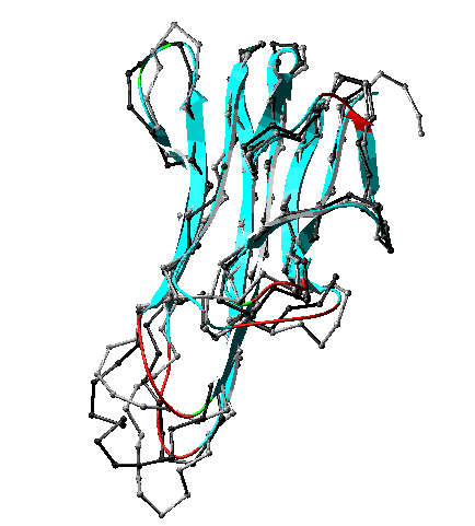
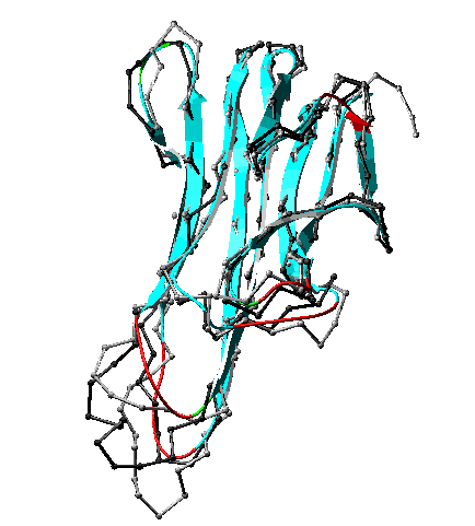
Homology model (ribbon) with two templates (gray and black). as returned from SWISS-MODEL and displayed in Swiss-PdbViewer. Ribbon model colored by confidence factor. Fit to templates is best in turquoise regions, poorest in red regions. The target protein is a fragment of FasL, a ligand for the widely expressed mammalian protein Fas. Interaction of Fas with FasL leads to rapid cell death via apoptosis. The template proteins are (1) tumor necrosis factor receptor P55, extracellular domain (PDB 1tnr, black) and (2) tumor necrosis factor-alpha (PDB 2tun, gray). The modeled FasL fragment is shown as ribbon and colored by model B-factors. Only the alpha carbons of the templates are shown. Convergent stereo.
A fixed value placed on a parameter during crystallographic refinement. For example, in early stages of refinement, all occupancies might be constrained to values of 1.0. In later stages, this constraint might be lifted and occupancies allowed to refine to non-unity values. The results might reflect alternative conformations of side chains, or partial occupancy of metal-ion binding sites. See crystallographic restraint.
We would like to ask whether a homology model is correct. Of course, we could say that it is correct if it agrees with the actual molecular structure. But we do not have this kind of assurance about any model, even one derived from experiment. It is more reasonable for us to define correct as agreeing to within experimental error with an experimental (X-ray or NMR) structure.
Typically, however, we want to use a homology model because it is all we have. In some cases, even without an experimental model for comparison, we can recognize incorrectness. A model is incorrect if it is in any sense impossible. What are signs of an incorrect model? One is the presence of hydrophobic side chains on the surface of the model, or buried polar or ionic groups that do not have their hydrogen-bonding or ionic-bonding capabilities satisfied by neighboring groups. Another is poor agreement with expected values of structural parameters like bond lengths and angles. Another is the presence of unfavorable noncovalent contacts or "clashes." Still another is unreasonable conformational angles, as exhibited in a Ramachandran diagram.
We know that high-quality models from crystallography and NMR do not harbor these deficiencies, and we should not accept them in a homology model. Many molecular graphics programs can compute deviations from expected bond geometry; highlight clashes with colors, dotted lines, or overlapping spheres; and display Ramachandran diagrams, thus giving us immediate visual evidence of problems with models.
We can also say that the model is incorrect if the sequence alignment is incorrect or not optimal. We can test the alignment of target with templates by using different alignment procedures, or by altering the alignment parameters to see if the current alignment is highly sensitive to slight changes in method. If so, it should shake our confidence in the model.
The original data in macromolecular structure determination by single-crystal X-ray crystallography are the measured positions and intensities of reflections in the diffraction pattern produced by the macromolecular crystal. Progress in structure determination requires learning the relative phases of the waves that produced the diffraction pattern, and then computing -- from positions, intensities, and phases of all the reflections -- an electron-density map of the molecule. Finally, a model is built to fit this map, a process called map interpretation.
Initial electron-density maps, calculated from data plus the first estimates of phases, are difficult to interpret, and only partial or low-resolution models can be built. These models are used to compute better estimates of phases, and from them, better maps. This iterative refinement process eventually converges to a clear map and a model that fits the map well.
The original data in macromolecular structure determination by NMR are very high-resolution multidimensional NMR spectra collected so as to reveal correlations between atoms that lie within a few bonds of each other (J coupling) or within a short distance of each other through space (NOE coupling). J couplings reveal local conformations, while NOE couplings reveal which parts of the protein are brought near each other by folding. Progress in structure determination requires assigning NMR resonances to specific atoms in the macromolecule, and then assigning couplings to pairs or groups of atoms. These couplings are used to produce a list of restraints that, in effect, demand that certain atoms in the final model be near each other or in specific conformational relationships to each other.
Once resonances and couplings have been assigned, a computer algorithm folds a model of the polypeptide from a random conformation into one that fits all the restraints and is also chemically reasonable. See Refinement (NMR).
Disordered regions of molecules exhibit themselves in crystallography as weak regions of electron density and as regions with high temperature factors. In NMR spectroscopy, disordered regions result in a dearth of structural restraints and high variability among the models in the ensemble. Atom positions in disordered regions are highly uncertain.
An electron-density map is, in a sense, the end-product of crystallographic structure determination. Simply put, the map is an image of the electron clouds surrounding the molecule. In a process called map interpretation, the crystallographer builds a model to fit this image.
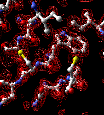
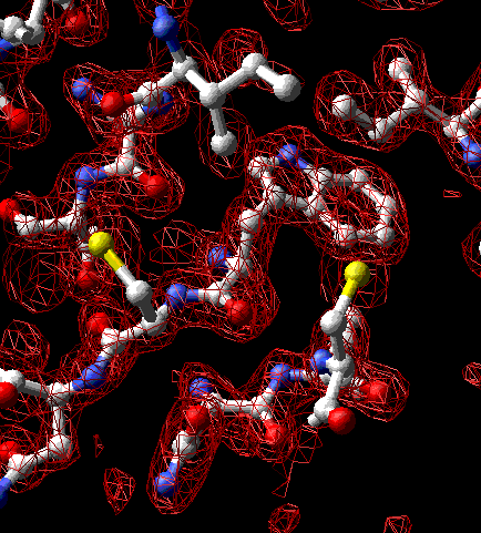
Thin section of electron-density map of lysozyme (PDB 1hel) centered at tryptophan-63. The molecular model is an interpretation of this map. Convergent stereo.
NMR structure determination entails building models that comply
with structural restraints obtained by analysis of J or NOE
couplings. Half a dozen to several dozen models are built in order to
see the full variety of models that fit all restraints. The resulting
set of models is called an ensemble (see figure below). A
single model is
usually derived by averaging atom positions and then minimizing the
energy of the resulting model. Both the ensemble coordinates and the
averaged model coordinates are usually available from the Protein
Data Bank. See Which model to
use.
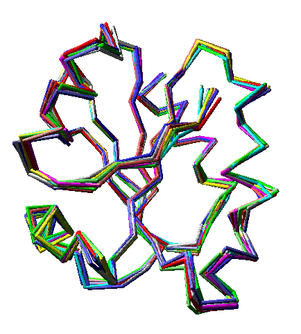
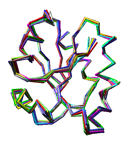
Ten models, each a different color, from an ensemble file (PDB 4trx) containing 33 models of human thioredoxin. Note that in some regions the models vary noticeably, while in others the are superimposed on each other almost perfectly. Only alpha carbons are shown. Convergent stereo.
The products of "structure determination" by diffraction methods (primarily single-crystal X-ray crystallography) and NMR spectroscopy are referred to as experimental models, in contrast with theoretical models, which include homology models and those obtained by simulation of folding or molecular dynamics. See Model versus structure.
First, see R-factor. R-factors are measures of the extent to which a crystallographic model accounts for the original experimental data -- specifically, the measured intensities of reflections in the diffraction pattern. As such, R-factors are important indicators of progress in refining models, and the final values of R-factors are important criteria of model quality.
The free R-factor, Rfree, is computed in the same manner as R, but using only a small set of randomly chosen intensities (the "test set") which are set aside from the beginning and not used during refinement. They are used only in the cross-validation or quality control process of assessing the agreement between calculated (from the model) and observed data. At any stage in refinement, Rfree measures how well the current atomic model predicts a subset of the measured reflection intensities that were not included in the refinement, whereas R measures how well the current model predicts the entire data set that produced the model.
Many crystallographers believe that Rfree gives a better and less-biased measure of refinement progress. In many test calculations, Rfree correlates very well with phase accuracy of the atomic model. In general, during intermediate stages of refinement, Rfree values are higher than R, but in the final stages, the two often become more similar. Because incompleteness of data can make structure determination more difficult (and perhaps because the lower values of R are somewhat seductive during stages where some encouragement is welcome), some crystallographers at first resisted using Rfree. But many now use both Rs to guide them in refinement, looking for refinement procedures that improve both, and proceeding with great caution when the two criteria appear to be in conflict.
The symmetry of functional macromolecular complexes in solution is sometimes important to understanding their functions, as in the binding of regulatory proteins having twofold rotational symmetry to palindromic DNA sequences. Users of models should be careful to distinguish the crystallographic asymmetric unit from the functional unit, which the Protein Data Bank has dubbed the "biologically functional molecule." For example, the functional unit of mammalian hemoglobin is a complex of four subunits, two each of two slightly different polypeptides, called a and b. We say that hemoglobin functions as an a2b2 tetramer. In some hemoglobin crystals, the twofold rotational symmetry axis of the tetramer corresponds to a unit-cell symmetry axis, and the asymmetric unit is a single ab dimer. In other cases, the crystallographic asymmetric unit may contain more than one biological unit.
A means of estimating the overall or average precision of atom locations in a refined crystallographic model. At best, the Luzzati plot allows an estimate of the upper limit of error in atomic coordinates. The figure below shows four theoretical curves on a Luzzati plot.
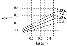
The numbers to the right of each smooth curve are theoretical estimates of the average uncertainty in the positions of atoms in the refined model (more precisely, the rms errors in atom positions). The average uncertainty has been shown to depend upon R-factors derived from the final model in various resolution ranges. To prepare data for a Luzzati plot, we separate the intensity data into groups of reflections in narrow ranges of 1/d (where d is the spacing of real lattice planes). Then we plot each R-factor (vertical axis) versus the midpoint value of 1/d for that group of reflections (horizontal axis). For example, we calculate R using only reflections corresponding to the range 1/d = 0.395 - 0.405 (reflections in the 2.53- to 2.47-Å range) and plot this R-factor versus 1/d = 0.400/Å, the midpoint value for this group. We repeat this process for the range 1/d = 0.385 - 0.395, and so forth. As the theoretical curves indicate, the R-factor typically increases for lower-resolution data (higher values of 1/d). The resulting curve should roughly fit one of the theoretical curves on the Luzzati plot. From the theoretical curve closest to the experimental R-factor curve, we learn the average uncertainty in the atom positions of the final model. It has been claimed that Luzzati plots with the free R-factor give even better estimates of uncertainty in coordinates.
Some scientists argue for using the term structure to refer to the results of experimental methods, like X-ray crystallography and NMR spectroscopy, and the term model to refer to theoretical models, including homology models and those derived from simulations of folding, dynamics, and ligand binding. Other scientists, pointing out that molecular structure is not open to our direct view, are more comfortable with the term model for all results of attempts to know molecular structure. In this view, models, experimental or theoretical (an imprecise distinction itself), represent the best we can do in our diverse efforts to know molecular structure. All of us sometimes refer loosely to a model as a structure, and to the process of constructing and refining models as structure determination. But in the end, no matter what the method, we are trying to construct models that agree with, and explain, what we know from experiments that are quite different from actually looking at structure.
One of several parameters included in refinement. The occupancy nj of atom j is a measure of the fraction of molecules in the crystal in which atom j actually occupies the position specified in the model. If all molecules in the crystal are precisely identical, then occupancies for all atoms are 1.00. Occupancy is included among refinement parameters because occasionally two or more distinct conformations are observed for a small region like a surface side chain. The model might refine better if atoms in this region are assigned occupancies equal to the fraction of side chains in each conformation. For example, if the two conformations occur with equal frequency, then atoms involved receive occupancies of 0.5 in each of their two possible positions. By including occupancies among the refinement parameters, we obtain estimates of the frequency of alternative conformations, giving some additional information about the dynamics of the protein molecule. We also make the model more accurate, which contributes to progress in the refinement.
In crystallography, unlike microscopy, the term resolution simply refers to the amount of data ultimately used in structure determination. In contrast, the precision of atom positions depends in part upon the resolution limits of the data, but also depends critically upon the quality of the data, as reflected by the R-factor. Good data can yield atom positions that are precise to within one-fifth to one-tenth of the stated resolution. One means of estimating the average or overall precision of atomic positions is the Luzzati plot. Also see temperature factor.
See Rms deviations (rmsd) from average ensemble coordinate positions.
A measure of agreement between the crystallographic model and the original X-ray diffraction data. The crystallographer calculates from the model the expected intensity of each reflection in the diffraction pattern, and then compares these calculated "data" with the experimental data, which consist of measured positions and intensities. The R-factor is used to assess the progress of structure refinement, and the final R-factor is one measure of model quality.
The R-factor is calculated as follows:

In this expression, each |Fobs| is derived from the measured intensity of a reflection in the diffraction pattern, and each |Fcalc| is the intensity of the same reflection calculated from the current model. Values of R range from zero (perfect agreement of calculated and observed intensities) to about 0.6, the R-factor obtained when a set of measured intensities is compared with a set of random intensities. An R-factor greater than 0.5 implies that agreement between observed and calculated intensities is very poor, and many models with R = 0.5 or greater will not respond to attempts at improvement unless more data are available. An early model with R near 0.4 is promising, and is likely to improve with various refinement methods. A desirable target R-factor for a protein model refined with data to 2.5 Å is 0.2. Very rarely, small, well-ordered proteins may refine to R = 0.1, whereas small organic molecules commonly refine to better than R = 0.05. When R approaches about 0.15, it sometimes becomes possible to discern hydrogen atoms in electron-density maps. See Free R-factor.
Measure of the similarity between an electron-density map calculated directly from the model and one calculated from experimental data. This measure is often provided in the form of a graph of RSR values versus residue number, showing clearly which residues give best and worst agreement with the experimental electron-density map. RSR is an excellent model-validation tool, and is calculated as follows (rho's are electron density values at grid points that cover the residue in question. obs and calc refer to experimental and model electron density):
RSR is sometimes expressed as RSCC, for real-space correlation coefficient. The latter does not require that the two densities be scaled against each other, but for the model user, the difference is not important.
A measure of agreement among multiple measurements of the same (not symmetry-related -- see Rsymm) reflections, with the different measurements being in different frames of data or different data sets. Rmerge is calculated as follows (Ii is the ith intensity measurement of reflection h, and <I> is the average intensity from multiple observations):

Often, separate values of Rmerge are given for a) all the data and b) data from the last or highest-resolution shell. The latter allows the model user to evaluate the reliability of data at the highest resolution used.
A measure of agreement among the independent measurements of symmetry-related reflections in a crystallographic data set. Symmetry-related reflections should have identical intensities. If they do not, it suggests some type of measurement error.
Rsymm is calculated as follows (I and I with bar on top represent intensities of two symmetry-related reflections):

A common reason for high Rsymm is strong absorption of X-rays by the crystal. If the lengths of the X-ray paths through such a crystal is very different for two symmetry-related reflections, then absorption will be different for the two measurements. In some cases, data can be improved by correcting for crystal absorption.
A plot showing the main-chain conformational angles in a polypeptide. This diagram is used to find problems in models during structure refinement. The conformational angles plotted are phi, the torsional angle of the N-CA bond, defined by the atoms C-N-CA-C (C is the carbonyl carbon); and psi, the torsional angle of the CA-C bond, defined by the atoms N-CA-C-N. In this figure, phi = psi = 180° (convergent stereo).
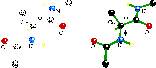
The pair of angles phi and psi of a single residue is greatly restricted by steric repulsion. The allowed pairs of values are depicted on a Ramachandran diagram as irregular polygons that enclose backbone conformational angles that do not give steric repulsion (yellow, inner polygons) or give only modest repulsion (blue, outer polygons). Every point (phi, psi) on the diagram represents the conformational angles phi and psi on either side of the alpha carbon of one residue. Each residue in the protein is represented with a dot or other mark on the plot.
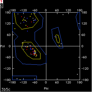
Ramachandran diagram for cytochrome b5 (PDB 3b5c). Small squares represent glycine residues; small crosses represent all others. Residues are colored by type: blue = positive, red = negative, yellow = polar, gray = nonpolar. Note that, in this very well-refined model, only glycines lie outside of allowed regions (blue polygons).
During the final stages of map fitting and crystallographic refinement, Ramachandran diagrams are a great aid in finding conformationally unrealistic regions of the model. Structure publications often include the diagram, with an explanation of any residues that lie in high-energy ("forbidden") areas. Glycines, because they lack a side chain, usually account for most of the residues that lie outside allowed regions. If nonglycine residues exhibit forbidden conformational angles, there should be some explanation, such as structural constraints that overcome the energetic cost of an unusual backbone conformation.
If a homology model appears to be correct (not harboring impossibilities such as clashing atoms) and accurate (fitting its templates well), we can also ask if it is reasonable, or in keeping with expectations for similar proteins. Researchers have developed several assessments of reasonableness that can sometimes signal problems with a model or specific regions of a model. One is to sum up the probabilities that each residue should occur in the environment in which it is found in the model. For all Protein Data Bank models, each of the 20 amino acids has a certain probability of belonging to one of the following classes: solvent-accessible surface, buried polar, exposed nonpolar, helix, sheet, or turn. Regions of a model that do not fit expectations based on these probabilities are suspect.
Another criterion of reasonableness is to look at how often pairs of residues interact with each other in the model in comparison to the same pairwise interactions in templates or proteins in general. The sum of pairwise potentials for the model, usually expressed as an "energy" (smaller is better) should be similar to that for the templates. One form of this criterion is called threading energy. Such criteria ask, in a sense, whether a particular stretch of residues is "happy" in its three-dimensional setting. If a fragment is "unhappy" by these criteria, then that part of the model may be in error.
To be meaningful, all assessments of reasonableness of the model must be compared with the same properties of the templates. After all, the templates themselves, even if they are high-quality experimental structures, may be unusual in comparison to the average protein.
Redundancy is calculated as
The calculation gives the average number of independent measurements of each reflection in a crystallographic data set. Two factors, symmetry and overlap, contribute to redundancy in a crystallographic data set. 1) The symmetry of the crystal results in the presence of equivalent reflections in different regions of reciprocal space. 2) The measurement of overlapping regions of the three-dimensional diffraction pattern, which is done to assure complete coverage, often results in multiple measurements of the same reflection. As a result of these two factors, a data set contains several independent measurements of each reflection. To improve accuracy in measuring reflection intensities, data collection strategies are intentionally designed to take advantage of symmetry and overlap to give redundancy of measurement. Such statistical parameters as standard deviation are used to measure agreement among the repeated measurements.
The iterative process of improving agreement between the molecular model and the crystallographic data. An important element in refinement is a computationally massive least-squares adjustment of 1) the atomic positions in the model, 2) occupancies, and 3) temperature factors in order to improve their agreement with 1) the data (reflection intensities), and 2) criteria of chemical reasonableness (structural parameters such as bond lengths and angles). The crystallographer might impose certain constraints and restraints on the model during refinement, often relaxing these restrictions as the refinement proceeds. Energy minimization may also be included in refinement. In the latter stages of structure determination, the crystallographer alternates between refinement and interpretation of the electron-density map. Signs of progress and ultimate success of refinement include 1) decreasing R-factor, 2) disappearance of residues from unfavorable regions of the Ramachandran plot, and 3) diminishing average deviation from ideal structural parameters.
The iterative process of improving agreement between the molecular model and NMR data. Protein structure determination by NMR ends with building a model of the protein that fits distance restraints from multidimensional NMR spectra. This is no trivial task. One general procedure entails starting from a model of the protein having the known sequence of residues, and having standard bond lengths and angles but random conformational angles. This starting structure will, of course, be inconsistent with most of the distance and conformational restraints derived from NMR. The amount of inconsistency can be expressed as a numerical parameter that should decline in value as the model improves, in somewhat the same fashion as the R-factor decreases as a crystallographic model's agreement with diffraction data improves during crystallographic refinement.
Starting from a random conformation, simulated annealing or some form of molecular dynamics is used to fold the model under the influence of simulated forces that maintain correct bond lengths and angles, provide weak versions of van der Waals repulsions, and draw the model toward allowed conformations, as well as toward satisfying the restraints derived from NMR. Electrostatic interactions and hydrogen-bonding are usually not simulated, in order to give larger weight to restraints based on experimental data; after all, we want to discover these interactions in the end, not build them into the model before the data have had their say.
The resulting model is examined for serious van der Waals collisions, and for large deviations from even one distance or conformational restraint. Models that suffer from one or more such problems are judged not to have converged to a satisfactory final conformation. They are discarded. The entire simulated folding process is carried out repeatedly, each time from a different random starting conformation, until a number of models (an ensemble) are found that are chemically realistic and consistent with all NMR-derived restraints. When the group of models appears to contain the full range of structures that satisfy all restraints, this phase of structure determination is complete. Finally, a single model, structurally averaged/energy minimized model, is derived from the ensemble. See Which model to use.
The number of measured reflections in a crystallographic data set, neglecting all repeated measurements of the same reflection or symmetry-related reflections. Repeated measurements of a reflection arise for reasons described under Redundancy. See Reflections, number of
The total number of measured reflections in a crystallographic data set, including all repeated measurements of the same reflection or symmetry-equivalent reflections. See Reflections, unique and Redundancy.
In X-ray crystallography, "2-Å model" means that the model takes into account diffraction from sets of equivalent, parallel planes of atoms spaced as closely as 2 Å in the unit cell. More closely spaced planes of atoms give rise to reflections farther from the center of the diffraction pattern. Presumably, data farther out than the stated resolution is unobtainable or too weak to be reliable. Although a final 2-Å electron-density map, viewed as an empty contour surface, may indeed not allow us to discern adjacent atoms at distance of 2Å or less, structural constraints on the model greatly increase the precision of atom positions. The main constraint is that we know we can fit the map with groups of atoms -- amino-acid residues -- having known connectivities, bond lengths, bond angles, and stereochemistry.
A subsidiary condition imposed on parameters during crystallographic refinement, such as the condition that all bond lengths and bond angles be within a specified range of values. See crystallographic constraint.
Atomic distances and conformational angles determined from NMR couplings or correlations. In NMR structure determination, the construction of a model complies with these restraints, resulting in a model that fits what NMR spectra say about which pairs of atoms are near each other through bonds or through space. An example of the effect of a restraint is shown in the figure below. There is NMR evidence that the amide hydrogen of Phe89 lies between 2Å and 5Å away from one of the side chain hydrogens ortho- to the beta carbon. The final model complies with this restraint, as shown by the dotted line between the two atoms.
Detail from NMR model of human thioredoxin (PDB 3trx) centered at phenyalanine-89. An single NOE correlation between the two atoms connected by a dotted line greatly limits the possible conformational relationships between the ring and the main chain. Convergent stereo.
The total number of distance and conformational restraints for an NMR model, divided by the number of residues in the model.
How much structural information must we obtain from NMR in order to derive reliable models? As summarized in the PDB file header for thioredoxin (PDB 3trx), the ensemble of 33 human thioredoxin models were determined from 1983 interproton distance restraints derived from NOE couplings, and 52 hydrogen-bonding distance restraints defining 26 hydrogen bonds. Finally, there were 98 phi and 71 psi backbone dihedral-angle restraints, and 72 CB-CG side-chain dihedral-angle restraints, derived from NOE and J coupling. Thus the conformation of each of the 33 final thioredoxin models is defined by a total of 2276 restraints. Thioredoxin contains 105 residues, so these models are based on about 22 restraints per residue. Very roughly speaking, an NMR model with over 20 restraints per residue is comparable to a 2.0-2.5 Å crystallographic model in the average precision of atomic positions.
A measure of how much the position of each atom in a model varies throughout the ensemble. The rmsd for an atom is the square root of the sum of squares of distances between that atom in all models in an NMR ensemble and the average position for that atom in the ensemble. The best quality models exhibit main-chain deviations no greater than 0.4 Å, with side-chain values below 1.0 Å. An averaged model can be colored according to this criterion (see Structurally averaged/energy minimized model). For emphasis: such coloring DOES NOT reflect the distances of averaged-model atoms from the average, but instead the amount of variation in atom positions in the ensemble.
A measure of how well the final crystallographic model conforms to expected values of bond lengths and bond angles. Expected values are derived from measurements of the same parameters in high-resolution models of small molecules. A high quality crystallographic model has rmsd values lower than 0.02 angstroms for bond lengths and lower than 4 degrees for bond angles. These values are restrained or constrained during parts of crystallographic refinement, so they are not as useful as quality indicators than parameters that are allowed to refine freely.
Designation of the symmetry of the unit cell of a crystal. Unit-cell symmetry guides the crystallographer in developing a data-collection strategy that will measure all unique reflections with the desired redundancy.
A single macromolecular model derived from an ensemble of NMR models by averaging atom positions and minimizing the energy (see figure below). See Which model to use.
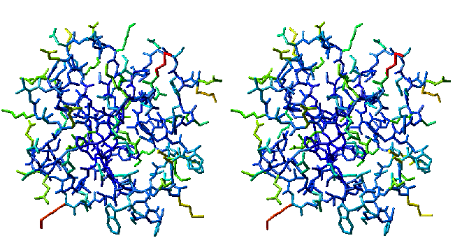
Structurally averaged/energy minimized model of human thioredoxin (PDB 3trx). Same orientation as the ensemble model above. Atoms are colored by atomic rms deviation of individual models about the mean atomic positions. Specifically, in red areas, the variation among the 33 models is greatest, and in blue areas, the variation among models is the smallest. Compare with the corresponding ensemble and note that red regions in this model correspond to ensemble regions where models show the greatest variation. Convergent stereo.
A general procedure is to compute the average position for each atom in the model and to build a model of all atoms in their average position. This model may be unrealistic in many respects. For example, bond lengths and angles involving atoms in their averaged positions may not be the same as standard values. This averaged model is then subjected to restrained energy minimization, which in essence brings bond lengths and angles to standard values, minimizes van der Waals repulsions, and maximizes noncovalent interactions, with minimal movement away from the averaged atomic coordinates.
Bond lengths, bond angles, and conformational angles in a model. These parameters are criteria of chemical reasonableness, and should approach accepted values during refinement. Refined models should exhibit rms deviations of no more than 0.02 Å for bond lengths and 4° for bond angles.
The temperature factor or B-factor can be thought of as a measure of how much an atom oscillates or vibrates around the position specified in the model. Atoms at side-chain termini are expected to exhibit more freedom of movement than main-chain atoms, and this movement amounts to spreading each atom over a small region of space. Diffraction is affected by this variation in atomic position, so it is realistic to assign a temperature factor to each atom and to include the factor among parameters to optimize during least-squares refinement.
From the temperature factors computed during refinement, we learn which atoms in the molecule have the most freedom of movement, and we gain some insight into the dynamics of our largely static model. In addition, adding the effects of motion to our model makes it more realistic and hence more likely to fit the data precisely.
If the temperature factor Bj is purely a measure of thermal motion at atom j, then in the simplest case of purely harmonic thermal motion of equal magnitude in all directions (called isotropic vibration), Bj is related to the magnitude of vibration as follows:
where {uj2} is the mean-square displacement of the atom from its rest position. Thus if the measured Bj is 79 Å2, the total mean-square displacement of atom j due to vibration is 1.0 Å2, and the rms displacement is the square root of {uj2}, or 1.0 Å. The B values of 20 and 5 Å2 correspond to rms displacements of 0.5 and 0.25 Å. But the B values obtained for most proteins are too large to be seen as reflecting purely thermal motion and must certainly reflect disorder as well.
Publications of refined structures often include a plot of average isotropic B values for side-chain and main-chain atoms of each residue. As an alternative, pictures of the model may be color coded by temperature factor: red ("hot") for high values of B and blue ("cold") for low values of B, as in the figure below. Either presentation calls the user's attention to parts of the molecule that are vibrationally active and parts that are particularly rigid. Not surprisingly, side-chain temperature factors are larger and more varied (5 - 60 Å2) than those of main-chain atoms (5 - 35 Å2).
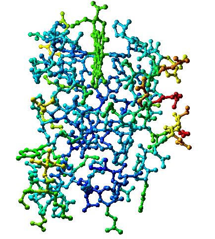
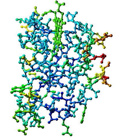
Cytochrome b5 (PDB 3b5c) colored by B-factors on relative scale -- highest B-factors red, lowest blue. The actual range of B-factors is 7.5 to 34, so all B-factors are relatively low. Convergent stereo.
Some publications also give the temperature factor of water molecules in the model, allowing the model user to evaluate the strength of evidence for their presence.
Some publications give average B-factors for main-chain atoms, for side-chain atoms, for observed residues, or for water molecules. Values for individual components of the model allow model users to find parts of the model most likely to harbor errors, making them more informative than average values.
A model derived from methods other than diffraction and NMR methods. The most common theoretical models are homology models. Other theoretical models are obtained from simulations of folding and molecular dynamics, and from "docking" experiments, in which researchers explore possible modes of interaction between experimental models (for example, protein-protein, protein-nucleic acid, or protein-ligand binding).
A criterion of reasonableness that reflects whether the environment of each residue in the model matches what is found for the same residue type in a representative set of protein folds. For a given residue, a small value of threading energy implies a reasonable environment for that residue type. Examples of residues that would have high threading energies are 1) a hydrophobic residue on the surface of a model, or 2) an ionic residue buried without compensating charge in a hydrophobic core.
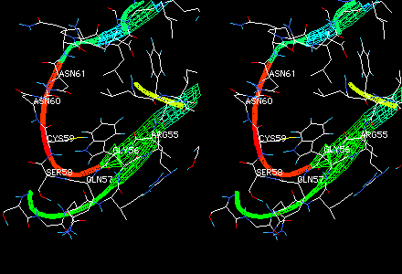
Region of high threading energy (red ribbon) in a homology model. A possible reason for high threading energy here is the presence of cysteine in a surface loop. Note in comparing this view with the full model that this is also a region of high model B-factor, and hence a low-confidence region. Convergent stereo.
Just as the auto mechanic sometimes has parts left over, electron-density maps occasionally show clear, empty density after all known contents of the crystal have been located. Apparent density can appear as an artifact of missing data, but this density disappears when a more complete set of data is obtained. Among the possible explanations for density that is not artifactual are ions like phosphate and sulfate from the mother liquor; reagents like mercaptoethanol, dithiothreitol, or detergents used in purification or crystallization; or cofactors, inhibitors, allosteric effectors, or other small molecules that survived the protein purification. Later discovery of previously unknown but important ligands has sometimes resulted in subsequent interpretation of empty density.
The dimensions of the unit cell, including lengths (in angstroms) of unit-cell edges a, b, and c, and the angles alpha, beta, and gamma between them. This information, like the space group, is primarily of interest to crystallographers.
The number of ordered water molecules added to the crystallographic model during refinement. The electron-density map can be improved if ordered waters can be found and added appropriately to the model. The number of ordered waters is usually about one water per residue of protein. If the number is far less than this, the model may be incompletely refined. If the number is far more, erroneous waters may have been placed in electron-density noise, and the model may harbor other errors as well.
At first glance, the structurally averaged/ energy minimized model would appear to serve most researchers who are looking for a molecular model to help them explain the function of the molecule and rationalize other chemical, spectroscopic, thermodynamic, and kinetic data. On the other hand, you might think that the ensemble and distance-restraint lists are of most use to those working to improve structure determination techniques. There are good reasons however, for all researchers to look carefully at the ensemble.
If some or all of the ensemble conformations reveal actual alternative conformations in solution, then these models contain useful information that may be lost in producing the averaged model. If the most important conformations for molecular function are represented in subsets of models within the final ensemble, then an averaged model may mislead us about function.
Models are are not molecules observed. No matter how they are obtained, before we ask what they tell us, we must ask how well macromolecular models fit with other things we already know. A model is like any scientific theory: it is useful only to the extent that it supports predictions that we can test by experiment. Our initial confidence in it is justified only to the extent that it fits what we already know. Our confidence can grow only if its predictions are verified.
